Introducing

Hunting Anomalies in the Stock Market

Nov 5, 2024

In this tutorial, we'll explore a method for detecting short-lived statistical anomalies in historical US stock market data. By analyzing trading metrics, such as the number of trades executed, we can identify unusual patterns that may indicate significant market volatility events. I've been interested in this idea for a while and wanted to put forth a high-level workflow for using a simple statistical method to figure out what "normal" looks like and then quickly spot deviations.

To find these anomalies, we will download data, then we’ll build tools that not only help identify these anomalies using a lookup table, but will also provide a user-friendly web interface for exploring and visualizing them. This hands-on approach should enhance your understanding of data analysis for anomaly detection and offer an adaptable workflow.

What Is an Anomaly?

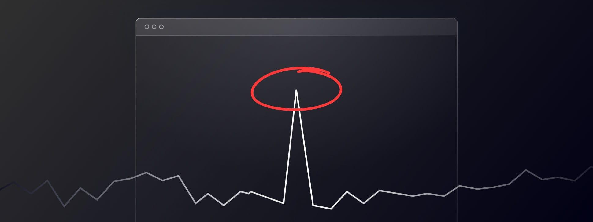
To find whether something is truly anomalous, we must first understand what "ordinary" looks like. This involves establishing a baseline or a pattern of life for a stock. This is similar to what you might have seen in a spy movie, where they have an interest in someone and start to follow them around to see what their daily routine is like. We'll do the same thing and start "following" stocks around to see what their daily routines are but at a market-wide level.

Let's look at some recent examples of detected anomalies using this method to give you a sense of what you can uncover. These examples represent some of the most significant deviations observed over the past few weeks, though as you’ll soon see many such events occur daily across the market.

Detecting anomalies is useful because sudden, short-lived deviations often indicate significant volatility events, which likely present potential trading opportunities. However, these events can also be extremely high-risk due to the unpredictable price movements since it’s easy to be on the wrong side. This tutorial focuses on the detection method and workflow for educational purposes only.

Getting Started

Before diving into the specifics of anomaly detection, we should probably cover the high-level workflow that guides our entire process. The steps include finding and downloading the right data, building a lookup table of pre-computed values (baselines) from the data, then querying the lookup table for deviations from the historical norms, and finally visualizing these anomalies for further analysis. This tutorial will walk you through each of these steps, ensuring you have a solid foundation for exploring stock market anomalies on your own.

Downloading Historical Data

There are a range of options when it comes to accessing financial data with Polygon.io: REST APIs for granular data into specific tickers, Flat Files for bulk download of market-wide historical data for things like backtesting (aggregates, trades, quotes, etc), and then real-time streaming data via WebSockets. For this tutorial, we'll focus on Flat Files because we can download many months worth of aggregated data across the entire market with just a few commands.

Before starting, you’ll need to confirm that you have an active Polygon.io subscription that includes Flat Files, or obtain an API key by signing up for a Stocks paid plan. This tutorial will use the MinIO client, compatible with S3 protocols, for managing and downloading data files from our S3 server. Detailed configuration guides for various S3 clients are available in our knowledge base article.

Download and install the MinIO client from the official page. Configure it using your polygon.io API credentials:

mc alias set s3polygon https://files.polygon.io YOUR_ACCESS_KEY YOUR_SECRET_KEY

List the available data files to understand what's accessible:

mc ls s3polygon/flatfiles/us_stocks_sip/day_aggs_v1/2024/

Download the daily aggregates for specific months you’re interested in:

mc cp --recursive s3polygon/flatfiles/us_stocks_sip/day_aggs_v1/2024/08/ ./aggregates_day/
mc cp --recursive s3polygon/flatfiles/us_stocks_sip/day_aggs_v1/2024/09/ ./aggregates_day/
mc cp --recursive s3polygon/flatfiles/us_stocks_sip/day_aggs_v1/2024/10/ ./aggregates_day/

Decompress the downloaded gzipped files for analysis:

gunzip ./aggregates_day/*.gz

We should now have all the daily aggregate CSV files uncompressed sitting in the aggregates_day/ directory. Here's as sample of what these file contain:

ticker,volume,open,close,high,low,window_start,transactions
A,2797662,142.24,142.86,144.22,141.75,1722484800000000000,36394
AA,17183234,32.95,31.47,33.27,31.09,1722484800000000000,59040
AAA,4428,25.0593,25.0449,25.075,25.0301,1722484800000000000,89
AAAU,3187275,24.27,24.165,24.3411,24.08,1722484800000000000,4379
AACG,8163,0.6601,0.651,0.6612,0.651,1722484800000000000,48
AACI,106098,8.31,10.45,11.63,8.31,1722484800000000000,1309
AACIU,615,10.99,10.99,10.99,10.99,1722484800000000000,23
AACT,22655,10.745,10.745,10.75,10.74,1722484800000000000,65
AACT.WS,2040922,0.125,0.099025,0.1412,0.0754,1722484800000000000,220

Having downloaded the historical data, the next section will walk you through building a lookup table of pre-computed values based on this historical data.

Building a Lookup Table

In this section, we use Python, along with the

and libraries, to construct a lookup table that stores the historical average number of trades and their standard deviations over a rolling window of the past 5 trading days for each stock. This pre-computed reference table enables quick identification of anomalies in trading data.

This method leverages a concept akin to hash tables in verification systems, where values are pre-computed for fast retrieval. We apply this to financial data to discern normal trading activity from short-term volatility spikes, which could indicate market anomalies. The code for all of the examples is located in this github repo.

Here’s the python

script to build the lookup table:

import os
import pandas as pd
from collections import defaultdict
import pickle
import json

# Directory containing the daily CSV files
data_dir = './aggregates_day/'

# Initialize a dictionary to hold trades data
trades_data = defaultdict(list)

# List all CSV files in the directory
files = sorted([f for f in os.listdir(data_dir) if f.endswith('.csv')])

print("Starting to process files...")

# Process each file (assuming files are named in order)
for file in files:
    print(f"Processing {file}")
    file_path = os.path.join(data_dir, file)
    df = pd.read_csv(file_path)
    # For each stock, store the date and relevant data
    for _, row in df.iterrows():
        ticker = row['ticker']
        date = pd.to_datetime(row['window_start'], unit='ns').date()
        trades = row['transactions']
        close_price = row['close']  # Ensure 'close' column exists in your CSV
        trades_data[ticker].append({
            'date': date,
            'trades': trades,
            'close_price': close_price
        })

print("Finished processing files.")
print("Building lookup table...")

# Now, build the lookup table with rolling averages and percentage price change
lookup_table = defaultdict(dict)  # Nested dict: ticker -> date -> stats

for ticker, records in trades_data.items():
    # Convert records to DataFrame
    df_ticker = pd.DataFrame(records)
    # Sort records by date
    df_ticker.sort_values('date', inplace=True)
    df_ticker.set_index('date', inplace=True)

    # Calculate the percentage change in close_price
    df_ticker['price_diff'] = df_ticker['close_price'].pct_change() * 100  # Multiply by 100 for percentage

    # Shift trades to exclude the current day from rolling calculations
    df_ticker['trades_shifted'] = df_ticker['trades'].shift(1)
    # Calculate rolling average and standard deviation over the previous 5 days
    df_ticker['avg_trades'] = df_ticker['trades_shifted'].rolling(window=5).mean()
    df_ticker['std_trades'] = df_ticker['trades_shifted'].rolling(window=5).std()
    # Store the data in the lookup table
    for date, row in df_ticker.iterrows():
        # Convert date to string for JSON serialization
        date_str = date.strftime('%Y-%m-%d')
        # Ensure rolling stats are available
        if pd.notnull(row['avg_trades']) and pd.notnull(row['std_trades']):
            lookup_table[ticker][date_str] = {
                'trades': row['trades'],
                'close_price': row['close_price'],
                'price_diff': row['price_diff'],
                'avg_trades': row['avg_trades'],
                'std_trades': row['std_trades']
            }
        else:
            # Store data without rolling stats if not enough data points
            lookup_table[ticker][date_str] = {
                'trades': row['trades'],
                'close_price': row['close_price'],
                'price_diff': row['price_diff'],
                'avg_trades': None,
                'std_trades': None
            }

print("Lookup table built successfully.")

# Convert defaultdict to regular dict for JSON serialization
lookup_table = {k: v for k, v in lookup_table.items()}

# Save the lookup table to a JSON file
with open('lookup_table.json', 'w') as f:
    json.dump(lookup_table, f, indent=4)

print("Lookup table saved to 'lookup_table.json'.")

# Save the lookup table to a file for later use
with open('lookup_table.pkl', 'wb') as f:
    pickle.dump(lookup_table, f)

print("Lookup table saved to 'lookup_table.pkl'.")

Here’s what running the script looks like:

$ python3 build-lookup-table.py
Starting to process files...
Processing 2024-08-01.csv
Processing 2024-08-02.csv
…
Processing 2024-10-17.csv
Processing 2024-10-18.csv
Finished processing files.
Building lookup table...
Lookup table built successfully.
Lookup table saved to 'lookup_table.pkl'.

$ du -h lookup_table.pkl
 80M	lookup_table.pkl

This script processes the downloaded stock market data and builds a lookup table that, for each ticker, stores the pre-computed average number of trades and the standard deviation over the past 5 trading days, in a rolling window. This lets us quickly find short-lived anomalies in the data across the entire US stock market.

Identifying Anomalies

Now, let's leverage the power of our pre-built lookup table to query anomalies without needing the original source data. This approach significantly enhances performance, since querying the lookup table provides an extremely fast method to quickly look through large amounts of historical data and detect anomalies for each trading day. By leveraging this method, we bypass the time-consuming data processing steps and jump straight to analyzing potential market anomalies, making our analysis both faster and more scalable even for real-time detection. The code for all of the examples is located in this github repo.

Here’s the python

script to query the lookup table:

import pickle
import argparse

# Parse command-line arguments
parser = argparse.ArgumentParser(description='Anomaly Detection Script')
parser.add_argument('date', type=str, help='Target date in YYYY-MM-DD format')
args = parser.parse_args()

# Load the lookup_table
with open('lookup_table.pkl', 'rb') as f:
    lookup_table = pickle.load(f)

# Threshold for considering an anomaly (e.g., 3 standard deviations)
threshold_multiplier = 3

# Date for which we want to find anomalies
target_date_str = args.date

# List to store anomalies
anomalies = []

# Iterate over all tickers in the lookup table
for ticker, date_data in lookup_table.items():
    if target_date_str in date_data:
        data = date_data[target_date_str]
        trades = data['trades']
        avg_trades = data['avg_trades']
        std_trades = data['std_trades']
        if (
            avg_trades is not None and
            std_trades is not None and
            std_trades > 0
        ):
            z_score = (trades - avg_trades) / std_trades
            if z_score > threshold_multiplier:
                anomalies.append({
                    'ticker': ticker,
                    'date': target_date_str,
                    'trades': trades,
                    'avg_trades': avg_trades,
                    'std_trades': std_trades,
                    'z_score': z_score,
                    'close_price': data['close_price'],
                    'price_diff': data['price_diff']
                })

# Sort anomalies by trades in descending order
anomalies.sort(key=lambda x: x['trades'], reverse=True)

# Print the anomalies with aligned columns
print(f"\nAnomalies Found for {target_date_str}:\n")
print(f"{'Ticker':<10}{'Trades':>10}{'Avg Trades':>15}{'Std Dev':>10}{'Z-score':>10}{'Close Price':>12}{'Price Diff':>12}")
print("-" * 91)
for anomaly in anomalies:
    print(
        f"{anomaly['ticker']:<10}"
        f"{anomaly['trades']:>10.0f}"
        f"{anomaly['avg_trades']:>15.2f}"
        f"{anomaly['std_trades']:>10.2f}"
        f"{anomaly['z_score']:>10.2f}"
        f"{anomaly['close_price']:>12.2f}"
        f"{anomaly['price_diff']:>12.2f}"
    )

To analyze a specific date's data for anomalies, run the script with the date as an argument:

$ python3 query-lookup-table.py 2024-10-18

You can also pipe the data into a file like this:

$ python3 query-lookup-table.py 2024-10-18 > 2024-10-18.txt

The output lists stocks where the number of trades on the specified date significantly exceeded the norm, indicating potential market events or anomalies.

Anomalies Found for 2024-10-18:

Ticker        Trades     Avg Trades   Std Dev   Z-score Close Price  Price Diff
-------------------------------------------------------------------------------------------
VTAK          460548        6291.40  12387.12     36.67        0.91      106.49
PEGY          387360       15769.40  10026.18     37.06        8.15       47.91
NFLX          378687      125174.00  66580.70      3.81      763.89       11.09
JDZG          348468       37128.60  48356.15      6.44        2.09       22.94
CVS           309745       89486.00  25237.53      8.73       60.34       -5.23
HEPS          215693        1988.60    684.85    312.04        3.51       59.55
EFSH          188632        2416.40   2782.17     66.93        5.26      198.76
SLB           162587       79685.60  16971.32      4.88       41.92       -4.71
IONQ          160601      103573.60  16778.08      3.40       13.30        6.40
BIVI          159263         660.80    156.14   1015.78        2.35      109.82
...

Having queried the lookup table, we've successfully identified a list of anomalies based on specific criteria set for trading volumes. Now we can find potentially interesting market events or anomalies, yet the output merely lists these anomalies without letting us really see them. To fix this, the next section will introduce a web interface that overlays our lookup table. This tool enables us to select a specific day and then visually explore the detected anomalies events through aggregated candlestick data, hopefully providing a more intuitive understanding of the event by looking at the trading activity.

Exploring Anomalies with a Browser-Based Interface

To enhance the interactivity of our anomaly detection analysis tutorial, we have created a simple browser-based tool so that you can explore these anomalies directly through your web browser. This interface takes the next step and downloads the aggregated bars for the specific anomaly so that you can get a sense of what was happening.

Before launching the interface, ensure you have the following:

• Same as before, you'll need an API key from Polygon.io because we're going to be accessing the REST API that retrieves aggregated trading data for the tickers and dates of interest.
• The Polygon.io client-python library installed on your system, as it is used to fetch the necessary data on demand. If you followed earlier parts of this tutorial to download the data, you should already have this setup. The code for all of the examples is located in this github repo.

To start exploring the anomalies, run the interface script on your local machine:

python3 gui-lookup-table.py

After initiating the script, connect to the following URL in your web browser:

http://localhost:8888

The interface automatically loads the trading data for the last day seen, and you can navigate through time just as you would at the command line by specifying a date using the next and previous buttons. This feature allows you to explore anomalies over different days without manually altering script parameters.

Detected anomalies for the displayed date are listed within the interface. You can select any anomaly to delve deeper into its specifics. Upon selection, the interface will display an aggregated bar chart resembling candlestick charts used in financial analysis. This chart visually represents the trading activity of the day, highlighting the high, low, open, and close prices which can help you visually see what happened during that trading session.

The browser-based interface provides a hands-on way to visually compare and analyze the anomalies. By clicking through different dates and tickers, you can view detailed trading data including volume, price movements, and more. This visual representation aids in understanding the scale and impact of each anomaly, offering insights that are not easily discernible from raw data alone.

While this part of the tutorial does not dive into the specific coding details of the interface since it is a few hundred lines of code, it's important to note that the interface runs locally on your machine. It uses the pre-computed lookup table we built and accesses the Polygon.io API to dynamically provide aggregate bars for the ticker and date in question.

Next Steps

In this tutorial, we've explored the process of detecting short-lived anomalies in the stock market using polygon.io's extensive historical data with Flat Files. By downloading data, constructing a lookup table for rapid analysis, and employing a browser-based interface for interactive visualization, we've established a comprehensive workflow that not only identifies but also helps understand market anomalies.

Happy Anomaly Hunting!

• Justin

  editor

  Read More